Date - 04/09/2026
Session Five deliberately stopped the moment a first loss number appeared, leaving the training half of makemore part 2 for today. Every open question at the end of that session is an item in the first half of this one: the learning rate search, the three-way data split, and the embedding plot.
We paired that with a first proper look at retrieval-augmented generation, and the reason for the pairing is the last of those open questions. The video ends by plotting the two-dimensional embeddings and watching the vowels cluster together. That plot is nearest-neighbour search. Putting it one slide before a vector database doing the same thing in 1,536 dimensions makes the second half land in a way that starting retrieval cold would not.
So the session had two halves and one idea: putting meaning into a vector space, and getting it back out again.
The first half finished the model, sweeping for a learning rate instead of guessing, splitting the data three ways, and finally looking at the embedding table it had trained. The second half crossed over to retrieval: why RAG exists, the two pipelines, the three ways of finding a chunk, and why retrieval fails, which we demonstrated rather than described.
The connecting sentence, worth stating plainly: the first half trains a tiny embedding table from scratch, and the second half borrows an enormous one. The lookup is identical. Only the scale and the training objective change.
27 rows and 2 dimensions
In the systems we will actually ship, nobody trains the embedding. It gets called. Everything else is the same idea.
Part one — finishing the MLP
Finding a learning rate instead of guessing one
Session Four used 0.1 because it was a plausible number. That is not a method.
The method is to sweep in log space. Build a range of candidate rates spaced exponentially, run a step at each, plot the loss against the rate, and look at the shape of the curve.
lre = torch.linspace(-3, 0, 1000)   # exponents from -3 to 0
lrs = 10**lre                       # 0.001 → 1.0
Too small and the loss barely moves. Too large and it overshoots, so the loss climbs. Between the two is a valley, and the floor of that valley is the answer.
The reassuring part is that the useful region is wide. This is not a hunt for a precise value; it is a matter of avoiding two obviously wrong regimes, and a rough answer is enough.
There is also learning rate decay. Late in training, drop the rate by a factor of ten. The last portion of the loss comes from taking smaller steps — long strides get you to the neighbourhood, short ones find the door.
Three splits, three different jobs
A single split tells you very little. The point of having three is that each set answers a question the others cannot.
The training set, roughly eighty per cent of the data, fits the parameters. Gradients come from here and only from here.
The validation set, often called the dev set, is roughly ten per cent and chooses the hyperparameters: layer size, embedding dimension, learning rate. It is intended to be looked at often.
The test set, the remaining ten per cent, reports the honest number. It should be touched once, at the very end.
The reason for the third set is that every look at the test set burns a little of it. The moment anything is tuned on the basis of test performance, that set has quietly become a second validation set and the honest number is gone.
One reading of the numbers is easy to miss. When training loss and validation loss are roughly equal, the model is underfitting — it is too small, not overtrained. Everyone assumes that a gap means overfitting; almost nobody remembers that the absence of a gap is also information. With a 27 × 2 table and a hundred hidden neurons we are firmly in the too-small regime, which is exactly why the experiments with a larger hidden layer and a larger embedding size exist.
Looking at the embeddings
Plotting the twenty-seven characters as points in their two-dimensional space makes the structure visible. The vowels sit together. The dot, q, and the other oddballs sit apart on their own.
Nothing in the code, the dataset, or the loss function mentions vowels. The only pressure applied to those numbers was to predict the next character better. The clustering is a side effect of the prediction task and was never a goal.
That is the hinge of the whole session, and it is what makes the second half meaningful. You have just trained an embedding table. Now you borrow one.
Part two — retrieval-augmented generation
Why RAG exists
A model can be excellent at language and know nothing whatsoever about your organisation. Those are separable problems.
It never saw your data. Internal documents, tickets, contracts and wikis were not in the training set and never will be.
Your data changes weekly. A policy updated on Monday should be answerable on Monday, and retraining cannot move at that speed.
You need to show the source. An answer nobody can verify is worth very little in a business setting, and retrieval hands you the citation for free.
The question that always follows is why not simply fine-tune. Fine-tuning changes how the model writes: tone, format, structure. It is a poor and expensive way to teach new facts, and it provides no way to update or cite them. Retrieval changes what the model sees. Different tool, different problem. Style against facts is the one-line answer.
Two pipelines, not one
Almost every RAG bug turns out to be confusion about which of these two pipelines is being discussed.
The indexing pipeline runs offline, once per document: load, split into chunks, embed each chunk, store the vectors along with their metadata.
The query pipeline runs once per question: embed the question, run a similarity search, assemble the context, send it to the model.
The single most common silent failure is using one embedding model to index and a different one to query. That compares coordinates from two different spaces. Nothing raises an error. The results are simply meaningless.
Similarity search
Nearest neighbours by cosine distance in the embedding space. That is all it is — the same operation as the vowel plot from the first half, at 1,536 dimensions instead of two, where it can no longer be eyeballed.
Three ways to find a chunk
Everything above is semantic search, which is one of three mechanisms and is not always the right one.
Keyword search, typically BM25, matches the words themselves. It scores documents by how many of the query’s rare terms appear, weighted by how unusual each term is. There is no model and no vector involved; it is counting. It is strong on codes, identifiers, error strings and names, and blind to synonyms — a search for “car” will not find “automobile”.
Semantic search matches meaning. Both sides go through the embedding model and the vectors are compared, so the words need not overlap at all. It is strong on paraphrase, synonyms and vaguely worded questions, and blind to exact tokens that it has no reason to treat as special.
Metadata filtering matches structured fields with exact conditions, such as department = legal or year >= 2024. It is strong on scoping, permissions and freshness, and blind to anything about the text itself.
Metadata is not really a third kind of search, though. It narrows the candidate set without ranking it. Filtering and ranking are different operations, and conflating them is the source of a lot of confused pipeline design.
Spring AI’s VectorStore abstraction offers similarity search plus metadata filtering, but not BM25. True keyword or hybrid search is not part of the common interface, so hybrid search is left to the developer. The two options are dropping to the underlying store’s native client — Elasticsearch, OpenSearch or PGVector, with Azure AI Search having hybrid built in — or running the two queries separately and fusing the ranked lists.
Reciprocal rank fusion is the standard way to fuse them. Each document scores 1 / (60 + rank) in each list, and the scores are summed across lists, so a document ranking decently in both beats one that comes first in only one. No tuning is required. LangChain is further along here, with an EnsembleRetriever that pairs the two out of the box.
Chunking
Chunking is cutting a long document into pieces before embedding, because a whole book cannot be embedded as a single vector.
Fixed-size chunking cuts every N tokens. It is simple and it slices sentences in half. Structural chunking cuts on paragraphs or headings and respects meaning. A sliding window with overlap ensures that a sentence near a boundary still carries its surrounding context.
In Spring AI this is the text splitter stage of ingestion. TokenTextSplitter is the built-in fixed-size-with-overlap option. For structure-based splitting the reader itself does the work, with ParagraphPdfDocumentReader splitting on the PDF’s table of contents. Anything more sophisticated means writing a custom DocumentTransformer.
The point to take away is that whatever you cut is the unit you retrieve. Chunking is tuning, not configuration. The cut decides what it is even possible to retrieve. Too large and the relevant sentence is diluted by noise; too small and it is stranded without the context that explains it. It deserves considerably more attention than the ten seconds most tutorials give it.
Why retrieval fails
Everyone can explain how RAG works. Almost nobody explains why it does not. Having run one in production, this is the half that was free for us to teach and unavailable to most people covering this material, so it got the demonstration slot rather than a bullet list.
The first failure is that similarity is not relevance. The embedding measures whether two texts are about the same thing, not whether one answers the other. Ask “can I return a damaged item?” and a chunk reading “we do not accept returns on damaged items” scores beautifully. Same topic, same vocabulary, exactly the wrong answer. Opposites live very close together in embedding space, always. That is structural rather than a defect in any particular model.
The second failure is that exact terms vanish. Search for an error code such as ERR-409 and semantic search shrugs. It has no reason to treat that token as special, since it is a rare string with little learned meaning, so it does not pull strongly in any direction. This is the honest argument for hybrid search, and it is better felt than described.
The demonstration was one markdown file with things planted deliberately: one exact code, one policy line with its opposite sitting nearby, and a couple of long rambling paragraphs. Two queries against the existing application, with no new code. Proof that retrieval is the hard part.
Worth noting for anyone repeating this: the failures depend on the embedding model, so both queries need running beforehand to check that they actually break. A failure demonstration that accidentally succeeds is worse than no demonstration.
What to add when the baseline is not good enough
Reranking retrieves twenty candidates cheaply, then scores each one against the question using a smarter model and keeps the best three. It is cheap to add and it catches precisely the similarity-is-not-relevance cases that the embedding alone gets wrong.
Query rewriting handles questions that are vague or full of pronouns from three messages ago, rewriting them into a proper search query before embedding, sometimes into several.
Contextual retrieval prepends a short summary of the surrounding document to each chunk before embedding, so that no chunk is stranded without the context explaining it.
Hybrid search runs keyword and semantic side by side and fuses the two ranked lists. This is the large one, and the natural subject for the next session.
We deliberately left three things out and named them in a single slide as what the tutorials skip. Retrieval evaluation should be measured separately from answer evaluation, because a good answer from a bad retrieval is luck and the difference is invisible unless the two are measured apart. Access control must ensure that retrieval never returns a chunk the asking user is not cleared to see, which means filtering by permission at query time rather than hiding it in the prompt. And citations — “this came from section 4.2, page 14” — are cheap, since the metadata is already there, and are usually what makes users trust the system.
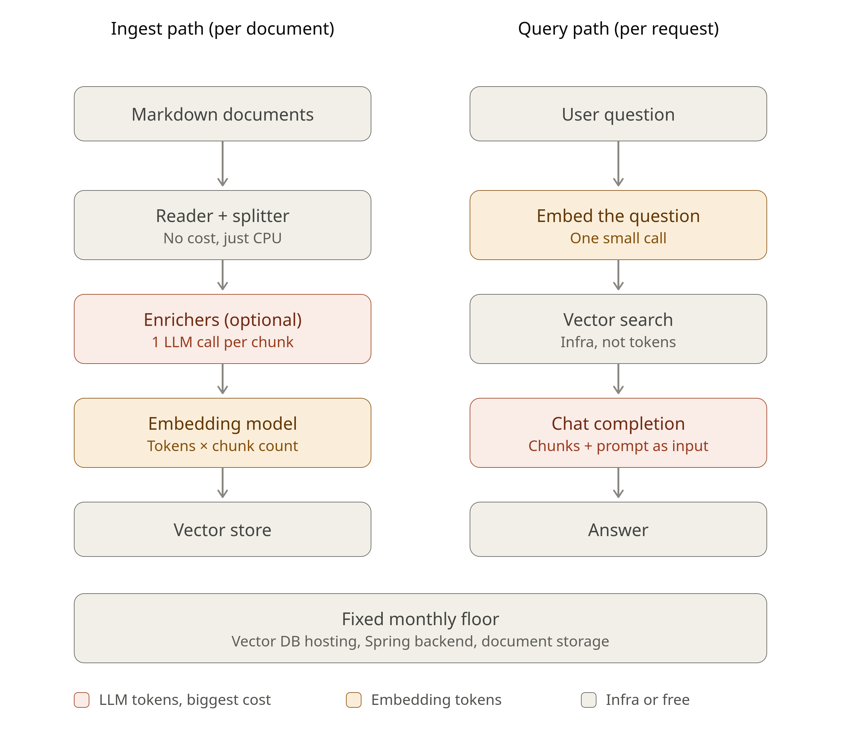
Vocabulary
- Learning rate decay — dropping the step size late in training to squeeze out the last of the loss
- Train, dev and test — fits the parameters, chooses the hyperparameters, reports the honest number once
- Underfitting — a model too small to capture the pattern; the tell is training and validation loss being roughly equal
- Indexing pipeline — load, split, embed, store; runs offline, per document
- Query pipeline — embed the question, search, assemble context, generate; runs per question
- Chunk — the unit a document is cut into, and therefore the unit that can be retrieved
- BM25 — keyword ranking by rare-term frequency, with no model and no vectors
- Cosine distance — the similarity measure behind nearest-neighbour search
- Reciprocal rank fusion — merging two ranked lists by summing
1 / (60 + rank) - Reranking — a second, smarter scoring pass over a cheaply retrieved candidate set
Where this fits for AI engineering
This is the session where the series stopped being preparation and became the job. The first half is the last of the from-scratch theory we planned to timebox. The second half is what we actually ship.
The two halves sitting in one hour is the argument we have been building toward since Session Three: you do not need to train models in order to build on them, but knowing what a trained embedding table actually is changes how you debug a retrieval pipeline.
The failure-modes half is also the part that could not have been taken from a tutorial. A generic chunk, embed and retrieve walkthrough is something anyone could deliver; why retrieval fails comes from having run one in production. That is a reasonable general rule for what belongs in these sessions — teach from the scar tissue rather than the tutorial.
Resources
- Andrej Karpathy — Building makemore Part 2: MLP (second half)
- Bengio et al. 2003 — A Neural Probabilistic Language Model
- makemore repository
- Spring AI documentation —
VectorStore,TokenTextSplitter,ParagraphPdfDocumentReader